
Rules on Graphs in Graphs of Rules, Part 2
In which I compare six ways to express the same rule logic in a graph of shapes

Rules are in the air. The pandemic boosted the gig economy, where, in search of new forms of governance, the interest in rules grew. At the same time, the second crypto boom occurred, which, in combination with increased social media power abuse, amplified interest in protocols; protocols are nothing more than rules that facilitate coordination. Since we can’t trust platforms (see what happened with Twitter), nor can we hope for special leaders to save us, it’s more likely that we need new rules.
The limits of new AI, such as LLMs, have prompted renewed interest in older AI (GOFAI), which was rule-based. The interest centers on how knowledge graphs support factual grounding, ontologies get a lot of new attention, but rules are rarely mentioned.
Rules help in dealing with various technical problems. Earlier this year, at a knowledge graph-based project, I proposed a solution to several challenges based on inference rules. At the Connected Data Conference in London, I shared how this was progressing and the benefits. Here are the slides. There is also a recording. I’ll touch upon some parts of that in the next part.
This post is part of a mini-series on inference rules, which is part of a larger series on rules, which is part of an even larger series about autonomy and cohesion.
The focus of this mini-series is inference rules working on knowledge graphs, where the rules are also stored in knowledge graphs, more specifically, using the Shapes Constraint Language (SHACL).
In the previous part, I used a ruleset of three rules attached to a single SHACL shape node to infer “has uncle” from “has parent” and “has brother”. That was done on a small example graph with nine nodes and eight edges. Now we are going to do it on a bigger graph, the represented relation in which are actual facts. We will also need one additional rule. More importantly, we’ll experiment with representing the same logic with different ruleset structures. From that, we can learn not only how to engineer SHACL-based rule graphs, but also that, even at this level, the dynamics between Autonomy and Cohesion can be observed.
Six different structures for the same logic
To test the same logic modelled with different rule connectivity, we’ll use a subgraph of Wikidata, containing people, their parents, and the siblings of their parents. Ignoring reverse relations and non-English labels, this gives a graph of over four million triples, which is sufficient for our purposes. You can run this query to generate that graph yourself from Qlever. In the last section, I’ll explain how to reproduce the whole experiment, step by step, including how to materialize this graph and run the different configurations of the rules graph on it.
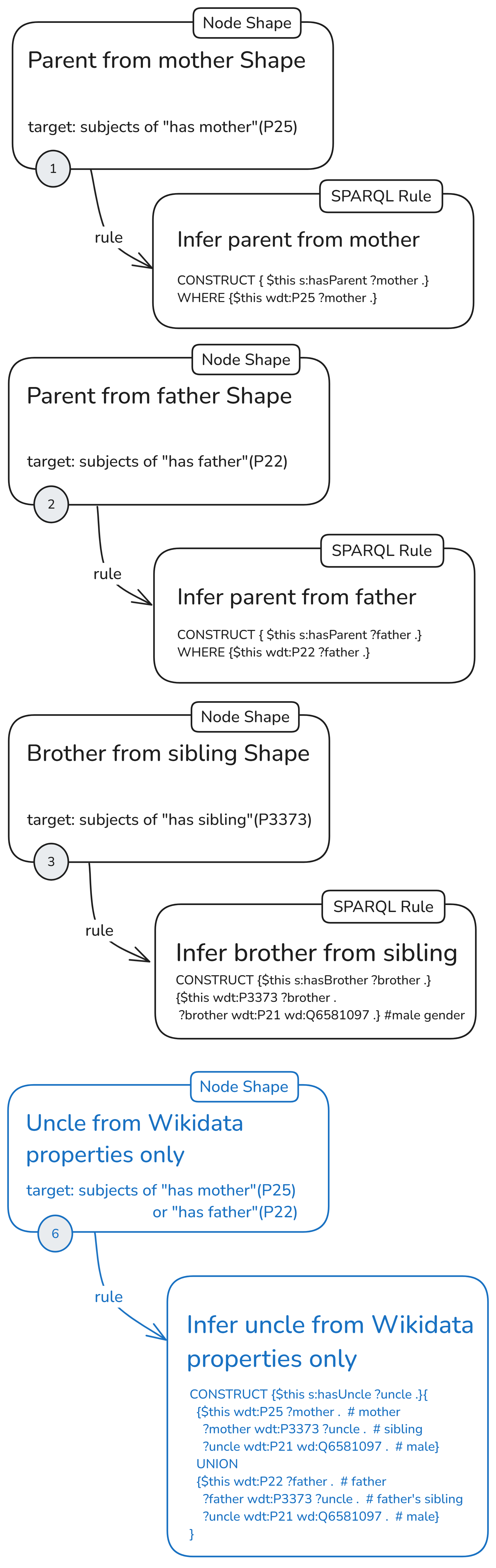
There are “mother” (P25) and “father” (P22) properties in Wikidata, which, to maintain the relational directionality, I’ll refer to as “has mother” and “has father.” There is no “has brother,” though, so we’ll need another rule in which to define “has brother” as any “sibling”(P3373) with “gender”(P21) “male” (Q6581097). That’s the additional rule I mentioned earlier.
There are more than a dozen ways to structure an SHACL graph with a ruleset that generates “has uncle” relations. I’ll pick six of them and will record the rule execution time so we can compare them.
Four rules, one shape
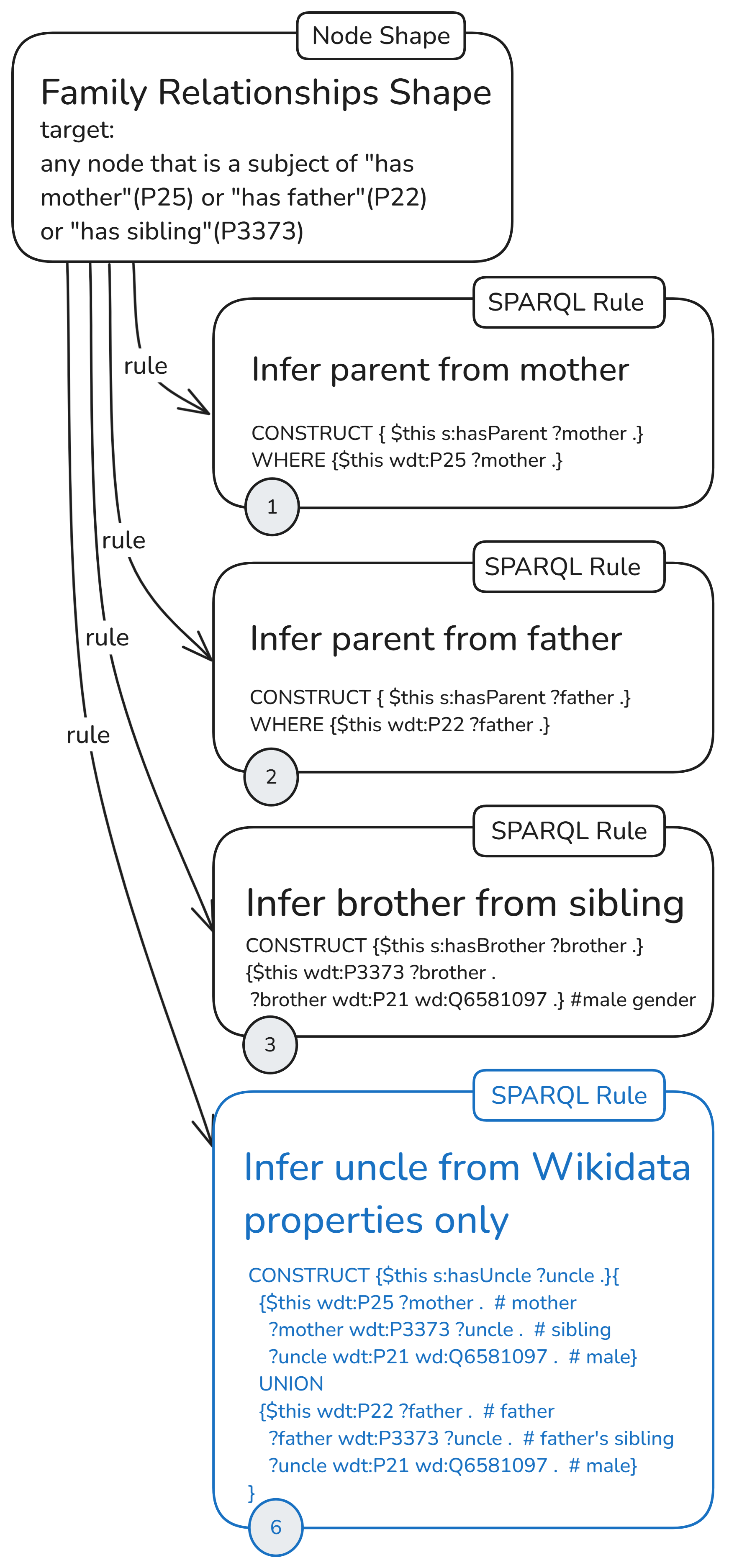
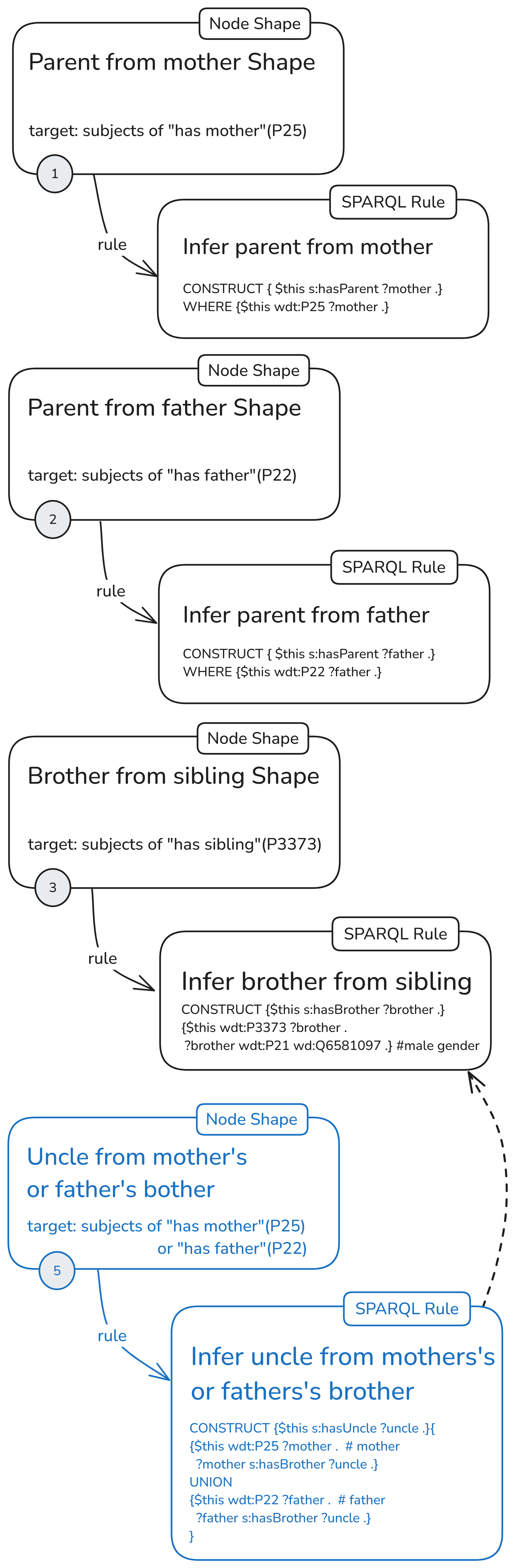
First, let’s start with a structure similar to the one used in the previous part, but this time with a variation of the rule for constructing uncle relations. We’ll use a single node shape to generate all nodes on which the four attached rules will be applied.
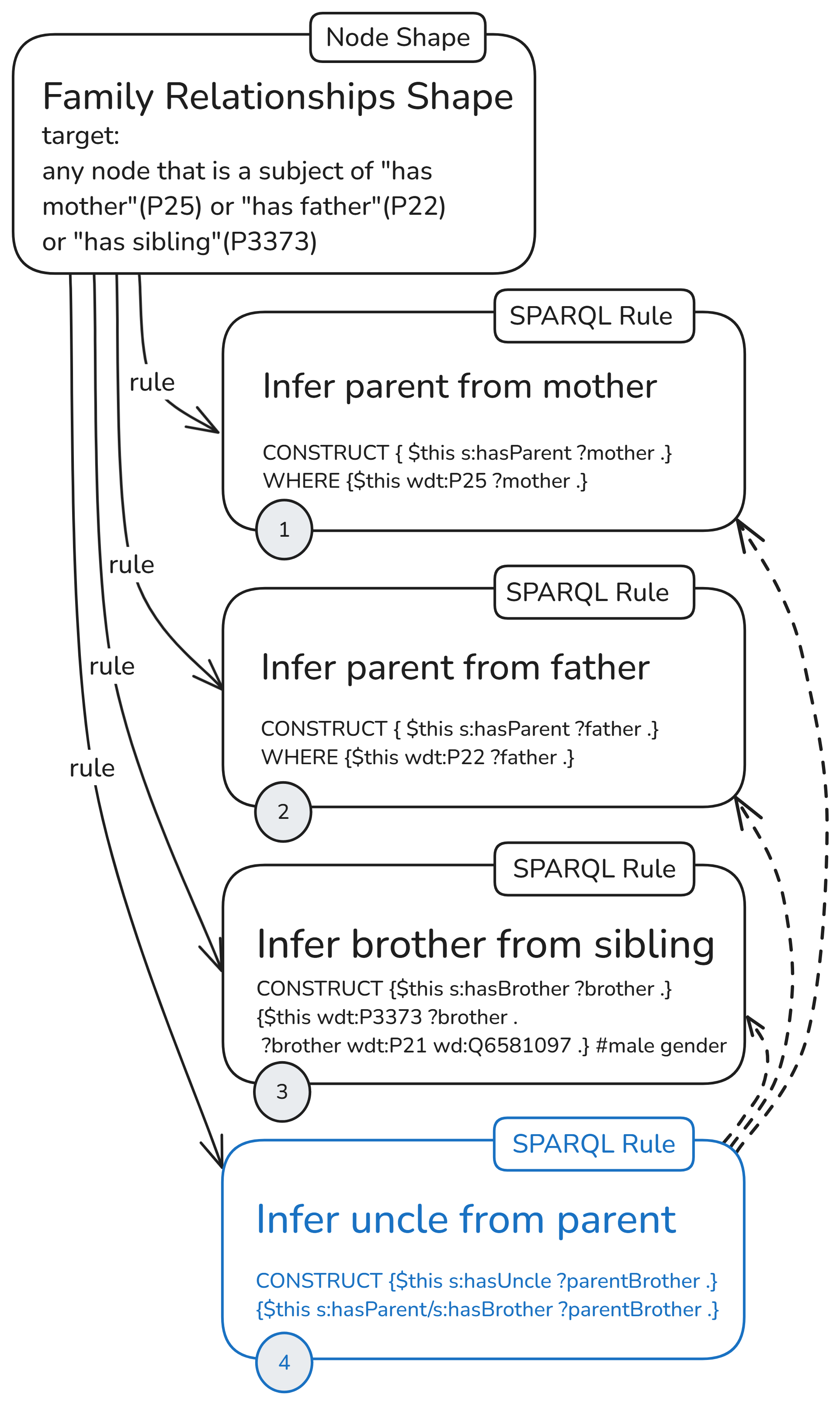
Since all rules are attached to one node shape, this node shape must specify the target nodes for all rules. The target nodes are the subjects of “has mother,” needed by the rule (1) to get “has parent,” the subject of “has father,” needed by the rule (2) to infer “has parent,” and the subject of “has sibling,” so that for those with gender male (Q6581097), it will construct “has brother” relations. During run time, these target declarations will produce the focus nodes that will be prebound to the $this variable in each rule.
What is specific about this initial rules setup is that the uncle rule (4) uses the output of the other three rules as input. It needs triples with “has parent” predicate, which are constructed by rules (1) and (2), and triples with “has brother” predicate, which are constructed by rule (3).
The dashed arrows show the rule dependencies. The solid line shows the actual sh:rule property in the graph, linking a node shape to an instance of sh:SPARQLrule. All other properties are not shown in the diagram. Of them sh:order and sh:deactivate are quite important, as you’ll see in the last section.
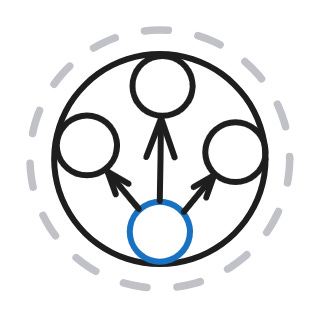
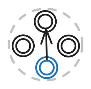
Later in this article, as a shorthand for this configuration with a single node shape and a fully dependent uncle rule, I’ll use the following icon:
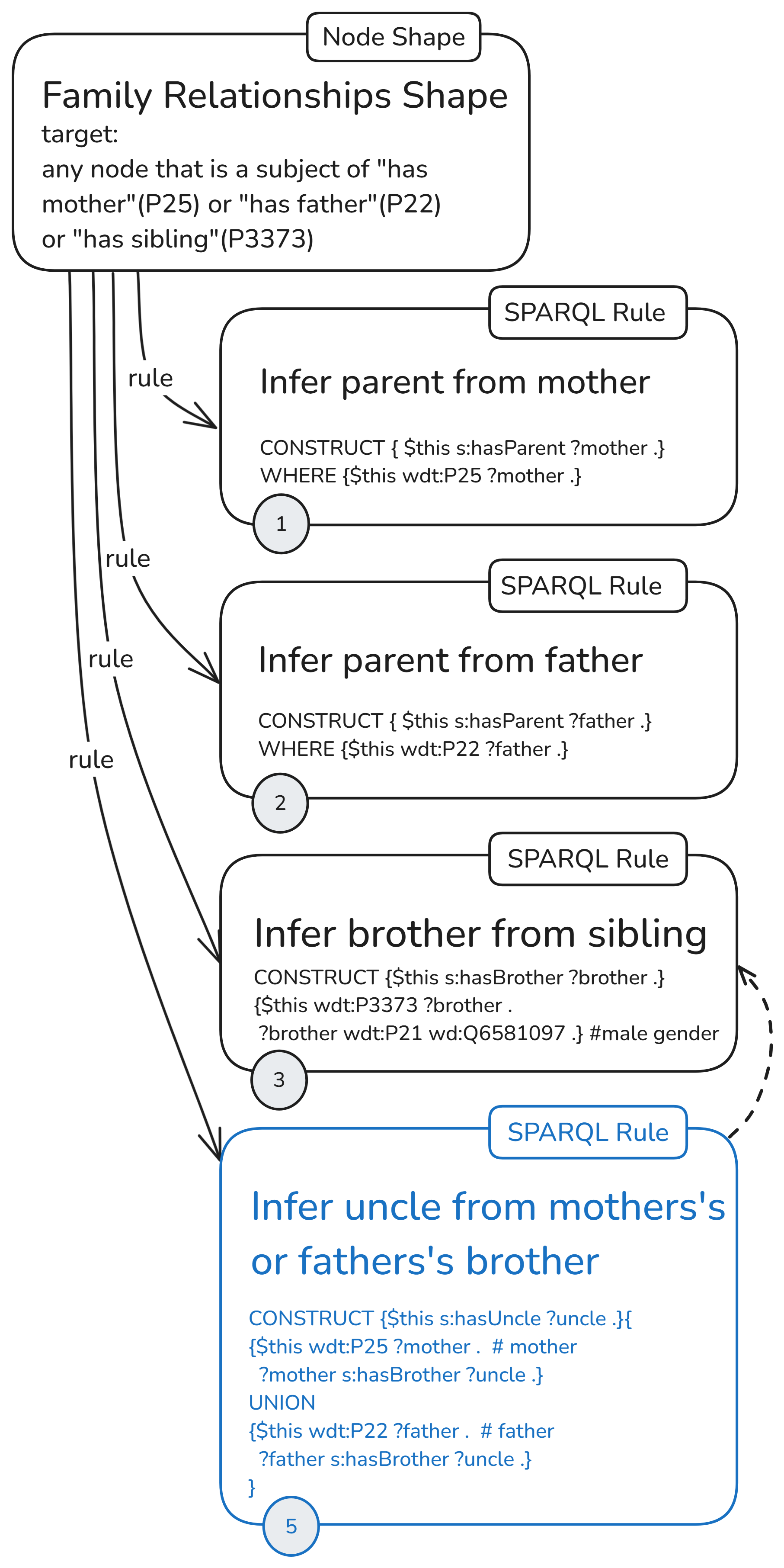
The next configuration follows the same overall logic and will generate triples with identical quality and quantity. This time, however, the uncle rule doesn’t use parent relations. It depends only on inferred brother relations and computes uncles from the property chains “has mother”—“has brother” and “has father”—“has brother.”
Another configuration can be such that the uncle rule computes “has brother” by itself but relies on rules (1) and (2) for “has parent.” As I wrote earlier, there are many possible ways to express the same rule logic. The point here was to pick one structure in which the uncle rule is neither fully dependent nor fully independent of the inferencing of the other rules.
Although the uncle rule no longer depends on the two parent rules, we keep them as they are. Why? First, they still provide useful shortcuts that speed up queries, and second, we need to maintain the same quantity and quality of inferred triples so we can compare the different structures of the rules graph.
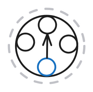
As a shorthand for this configuration with a single node shape and an uncle rule, dependent on one of the other rules, I’ll use the following icon:
In the last ruleset configuration with a single-node shape, the uncle rule (6) is independent of other rules. It doesn’t rely on inferred relations, only on asserted ones, and computes the uncle relationships by itself.
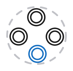
As a shorthand for this configuration with a single node shape and independent uncle rule, I’ll use the following icon:
Four rules, four shapes
Now, let's see what happens when each rule has its own node shape and that node shape targets only the nodes needed by that rule. The rules will be the same, and the three configurations will be of the same kind, where the uncle rule is fully dependent on the other two, semi-dependent (using only “has brother”), and completely independent. The main difference is that, whereas in the first three configurations, all rules depend on centralized focus node generation, in the second set of three configurations, focus-node generation is decentralized.
Here’s the first configuration. Again, it is made up of rules (1), (2), (3) and (4), but each one with its own node shape.
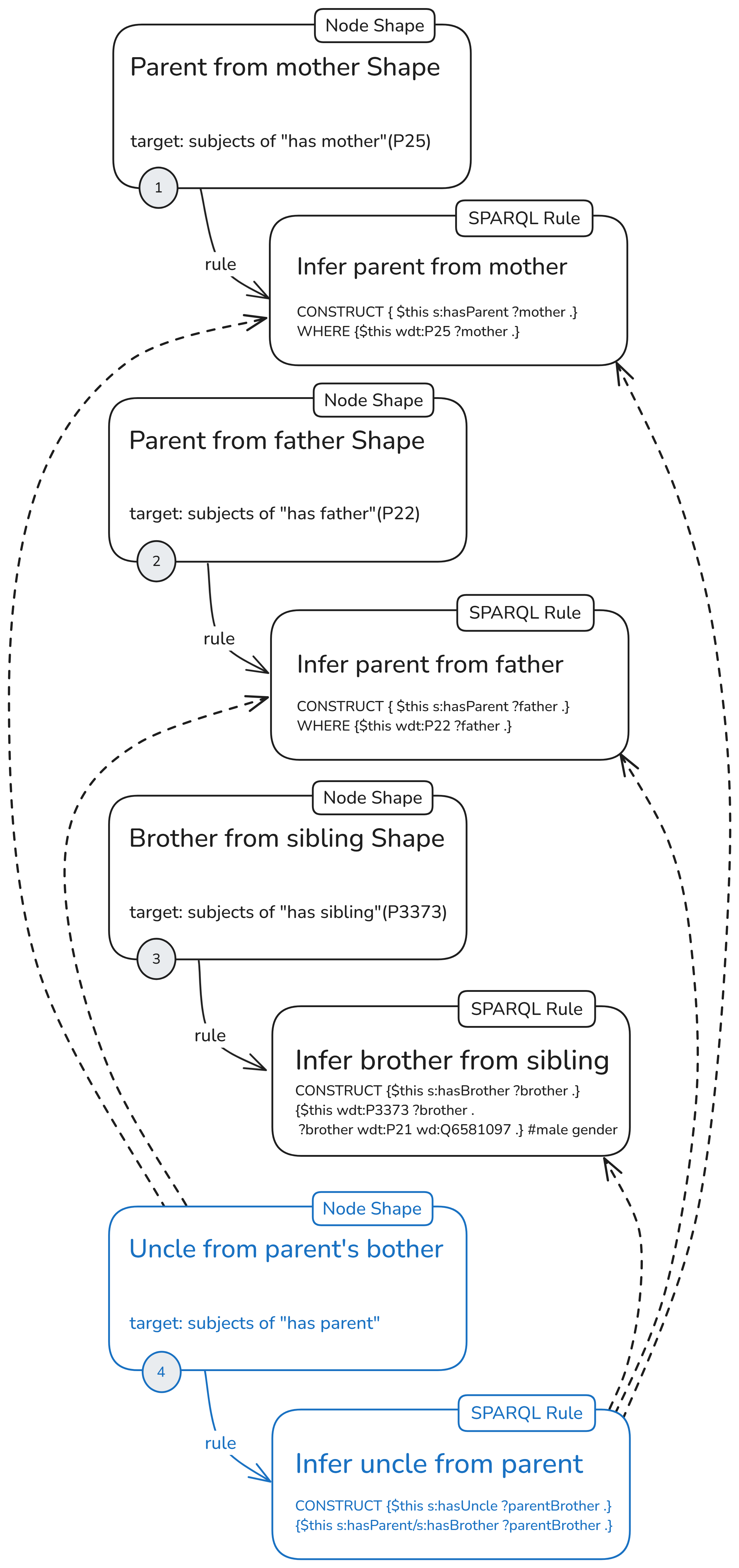
Now all the rules are applied to all and only the nodes generated by their node shapes. The uncle rule (4), as in the previous ruleset series, depends on the other three rules. Its node specifies its targets along an inferred property, so the generation of focus nodes here also depends on rules (1) and (2). Unlike the uncle rule, the node shape target depends only on these two (still, a lot) and not on rule (3), which infers “has brother” triples.
Here I have placed the numbers on the node shape, since, as you’ll see in the last section, deactivation is done at the node level, not at the rule level. The idea is that, since each node shape only produces targets for its own rule, when the rules are not used, it’s better to switch off the whole thing.
As a shorthand for this configuration with separate node shapes for each rule and an uncle rule, dependent on all other rules, I’ll use the following icon:
In the next configuration, we will use shape (5) to generate uncle relations. The rule of shape (5) depends only on the “has brother” triples inferred by rule (3).
Here, the node with the uncle rule does not depend on inferred triples to generate focus nodes.
As a shorthand for this configuration with separate node shapes for each rule and an uncle rule, dependent on one of the other rules, I’ll use the following icon:
In the last configuration, node shape (6) shares the same target, but its rule is independent, making the entire unit completely independent in the graph (excluding the prefix declarations; more on that later).
As a shorthand for this configuration with separate node shapes for each rule and a fully independent uncle rule, I’ll use the following icon:
Autonomy and Cohesion
Running all six configurations on the same graph produced the same number of triples, 192893, of which the same number of uncles, 19950 (if you decide to reproduce it, you may get different results, depending on when you run the query to extract the subgraph of Wikidata).
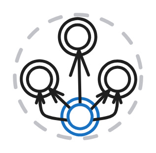
The result is basically a graph with “has parent,” “has brother,” and “has uncle” edges. Here’s one cluster of it:
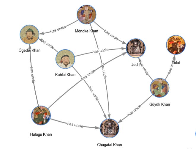
The number of parents, brothers, and uncles triples is the same, but because of the different structure and dependencies, it took a different time.
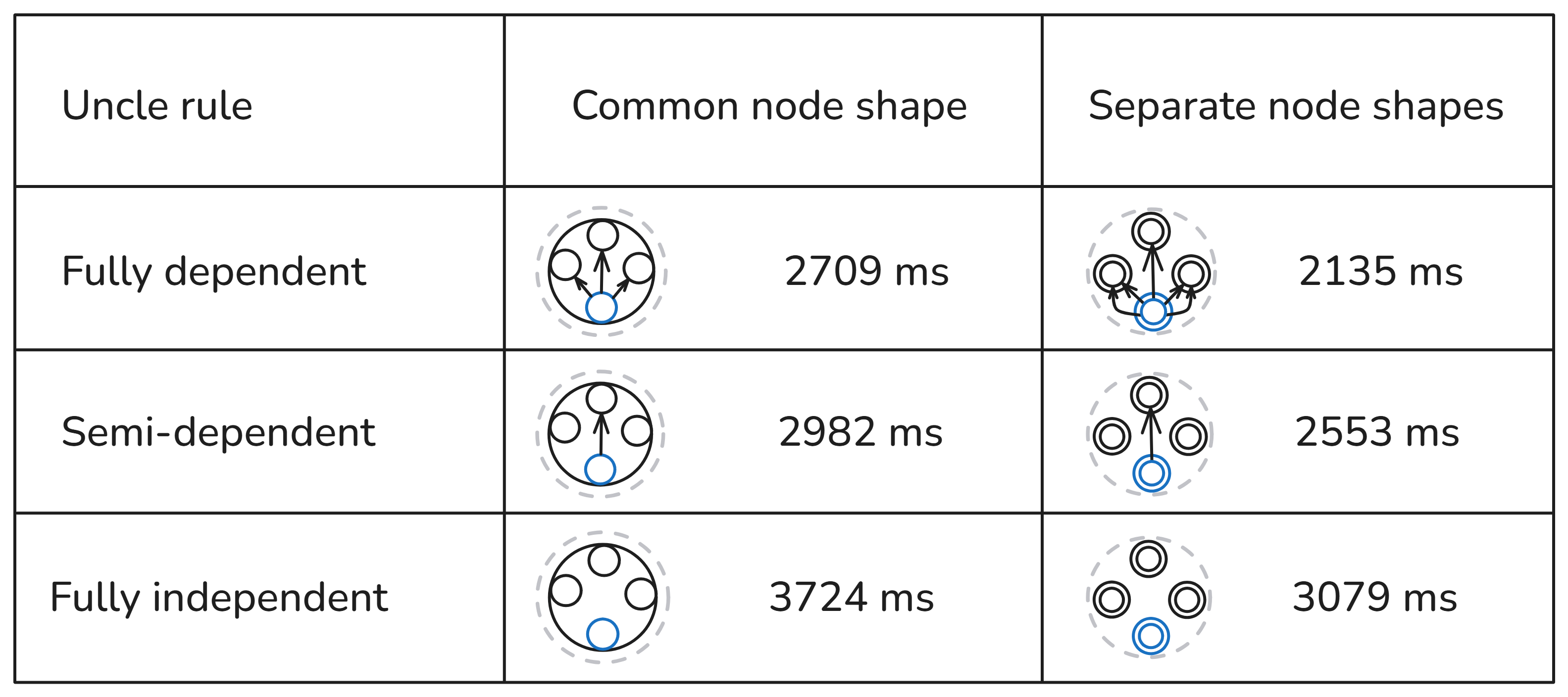
These results are interesting not only for what we can learn about SHACL-based rules graphs, but also for system engineering in general. To have a more useful comparison, apart from the performance perspective, or short-term efficiency, we need to add at least two long-term perspectives: cost of change and fault tolerance.
If we compare the two columns, we see that configurations with separate node shapes are consistently faster than configurations with a common node shape. From a SHACL-perspective, the reason is that the common node shape produces focus nodes for all the rules, so every rule is applied to a lot of targets, which, from the perspective of the rule conditions, are irrelevant. In contrast, the configuration with separate node shapes produces only the focus nodes, which are relevant to their rules.
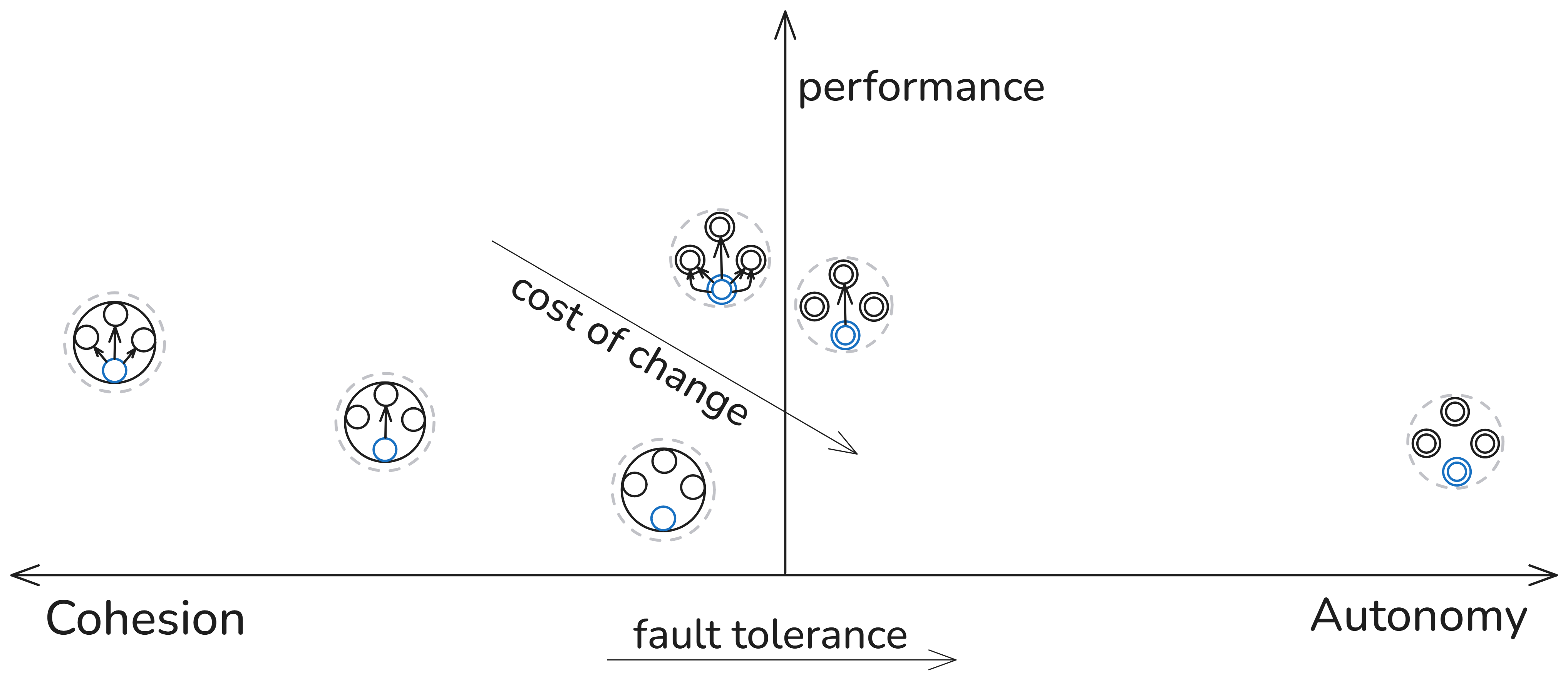
From a wider system perspective, the common node shape with rules 1-2-3-4 is imbalanced towards cohesion. Some of the cohesion results from extreme centralization. All rules depend on one node shape for their target nodes. The rules dependencies add even more cohesion: the uncle rule depends on the inferred triples generated by the other three rules. This makes the system vulnerable. A single bug in the targeting declaration will make the whole system collapse (manifested in this case in either giving an error or inferring zero triples). On top of that, if there is an error in any of the first three rules, the uncle rule will not work.
The 1-2-3-4 common shape node configuration needs to be excluded as an implementation option due to excessive cohesion (both structural and logical). The configuration 1-2-3-6 with separate node shapes also needs to be excluded for excessive “autonomy.” (I put autonomy in quotation marks, since in purely technical systems we can speak of “autonomy” only metaphorically as a proxy for degrees of freedom and decoupling, as discussed in another essay.)
The best-performing shape is the multi-shape 1-2-3-4 configuration, which produced all inferred triples in 2135ms (top-right cell in the table above). Not surprisingly, it’s one of those configurations where autonomy and cohesion are well balanced. There are separate node shapes for each rule (autonomy), but there is a lot of logical cohesion bringing efficiency. Once rules 1, 2, and 3 have run, the search space for rule 4 is highly optimized.
Apart from rule 4, depending on the output of the other three rules, its shape also depends on two of the rules, since there are no “has parent” subjects to target unless rules 1 and 2 are executed. So there is still more cohesion than necessary. This can be fixed by targeting the subjects of “has mother” and “has father”. The execution time is now 2514ms (not shown in the table). As expected, reducing this dependency has a performance cost. But that's probably a low price to pay for the increase in fault tolerance.
Yet, the multi-shape configuration with rules 1-2-3-5 has very good performance, second best, and very high fault tolerance. If the rules 1 and 2 don’t work because of an internal error or bad targeting of their node shapes, the uncle rule will still produce all uncle inferences.
What about the cost of change?
An easy way to measure it is to add two new requirements: include foster parents and infer also aunts, besides uncles. In both cases, the multi-shape 1-2-3-4 configuration will require minimal or no change to the uncle rule, whereas the multi-shape 1-2-3-5 configuration will require significant changes to the uncle rule, effectively duplicating other changes, such as adding new rules and modifying existing ones.
The final choice will depend on whether you prioritise modifiability (low cost of change), performance or resilience.
Fault tolerance generally increases with autonomy, at the cost of redundancy, in an approximately linear manner. The cost of change is not directly proportional to the increase in redundancy and depends on other factors. Yet in both series of configurations, those with rule 6 have a higher cost of change than those with rule 5, which have a higher cost of change than those with rule 4. But compared across the series, it’s not that straightforward. For example, the cost of some configuration changes with a single-node shape and rule 6 will be cheaper than implementing the same changes in a separate shape per rule and using rule 5 for uncles. For others, the cost of change will be lower in the multi-shape system.
Different ways of achieving cohesion bring different results. Some improve efficiency but make the system brittle, as is with the system in the left-most position on top. It may also introduce inefficiency. In the case of a SHACL system, such inefficiency may be manifested in the over-production of focus nodes, which increases the search space of SPARQL rules. But that is easily observed also in socio-technical systems, where the economy of scale is reduced by paying for a fat and inefficient bureaucracy.
Simply put, there is bad cohesion and good cohesion, and there is bad inefficiency and requisite inefficiency.
The focus of this part was on comparing different ways of structuring the graph of rules. In the next one, I’ll review some use cases and benefits.
Now, as promised, a step-by-step guide, including all the code used in this and the previous post.
Step by Step
Here’s how to reproduce the whole experiment.
Step 0: Tool
There are several open source tools you can use to run SHACL rules: the TopBraid SHACL API, its extended version, or pySHACL. Yet another open source SHACL tool, maplib, is currently adding SHACL rules.
For these two posts, I used TopBraid Composer Free Edition. It was discontinued in 2018, but the latest version is still available for download. I keep using it for training courses and workshops, since it has a GUI that makes it easy to run different experiments.
